Note: Synpi runs on Python 3.6+. Make sure your numpy version matches your python version.
In order to get started, first you need to install Synpi.
Click here to download Synpi.
After that, make a new python file and add the following code:
import synpi as spIf there are no errors, then it is installed correctly.
Now that there are no errors, let's make your first model.
Models in Synpi are found in the Core module. Models are defined as Sequential, this is because each layer in the model is executed sequentially. Sequential takes 1 parameter, a list. This list will contain all the layers for your model.
Your code should look like this:
import synpi as sp

model = sp.core.Sequential([])
That looks good, but we could make it a little nicer. Let's add some formatting so we can cleanly place are layers in the list.
import synpi as sp

model = sp.core.Sequential([
    #Our layers will go here
])
That's better!
Now let's add your first layers.
import synpi as sp

model = sp.core.Sequential([
    sp.layers.Linear(4, 8),
])
In this example, we have 1 Linear layer with 4 inputs and 8 outputs.
Lets try running an input through the model.
We'll make a dumby input with this line:
x = sp.mp.random.randn(1, 4)Next, we'll run it through the model using the forward method.
Example:
import synpi as sp

x = sp.mp.random.randn(1, 4)

model = sp.core.Sequential([
    sp.layers.Linear(4, 8),
])

output = model.forward(x)
Let's check the difference by printing the before and after.
print(x)
print(output)
It should look something like this:
Input: [[ 0.12096642 -0.07965834 -1.14641687 -2.18708405]]
Output: [[-2.06477941 -1.10365699 -1.67413473 -0.09623257 -0.84367984 -1.12725734 0.37240023 -1.35774596]]
As you can see, we had 4 inputs and 8 outputs came out.
Now lets add another layer.
import synpi as sp

x = sp.mp.random.randn(1, 4)

model = sp.core.Sequential([
    sp.layers.Linear(4, 8),
    sp.layers.Linear(6, 4),
])

output = model.forward(x)

print(x)
print(output)
Woah! This code will error!
As you can see the output of the first layer does not match the size of the input for the second layer.
They MUST match so the data can flow through the model.
Let's fix that.
import synpi as sp

x = sp.mp.random.randn(1, 4)

model = sp.core.Sequential([
    sp.layers.Linear(4, 8),
    sp.layers.Linear(8, 4),
])

output = model.forward(x)

print(x)
print(output)
Now, we have a model that flows like this:
4 inputs -> 8 outputs, 8 inputs -> 4 outputs
Our model should now have 4 outputs instead of 8.
Run the code and test it.
It should output something like this:
Input: [[0.98515768 0.39623649 0.47863461 1.07542597]]
Output: [[ 9.97256881  8.5809653  10.05421324 11.25969044]]
4 inputs, 4 outputs; Just like we predicted.
Next we'll add an activation layer to out model, right between our two linear layers.
model = sp.core.Sequential([
    sp.layers.Linear(4, 8),
    sp.activations.ReLU(),
    sp.layers.Linear(8, 4),
])
In the example we use the ReLU activation, but what is that?
The ReLU function takes an input. If that input is positive, the output is the input. If the input is negative, the output is 0.
Below is a graph of the ReLU function:
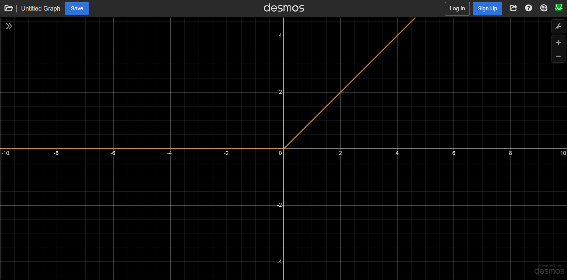
In the example we can't really see the effect of the ReLU layer. If you would like to, add another ReLU layer at the end of the model. There should be no negative outputs.
Next let's add an optimizer. Which optimizer we use changes how our models learns. We will be using ADAM.
model = sp.core.Sequential([
    sp.layers.Linear(4, 8),
    sp.activations.ReLU(),
    sp.layers.Linear(8, 4),
])
model.optimizer = sp.optimizers.ADAM(lr=0.001)
lr stands for learning rate and the bigger the learning rate the more aggressively it will train. Too high of a learning rate will result in large changes within the model that can make training unstable. If the learning rate is too low, the model will take forever to train.
Now that we have a decent structure for our model, let's train it!
First we need some multiple datapoints to train on. Let's go with 100.
In order to train the model, we need to tell it what the correct output should look like.
We will make some dumby data as a placeholder.
x = sp.mp.random.randn(100, 4)
y = sp.mp.random.randn(100, 4)
Next, we'll use the train function to train our model.
The train function takes a good bit of parameters, here they will be listed in order:
For this example, we are going to use the MSE loss function.
We are also going to set three other optional variables. We are going to set batch_size=1, talkback=True, and epochs=10.
import synpi as sp

x = sp.mp.random.randn(100, 4)
y = sp.mp.random.randn(100, 4)

model = sp.core.Sequential([
    sp.layers.Linear(4, 8),
    sp.activations.ReLU(),
    sp.layers.Linear(8, 4),
])
model.optimizer = sp.optimizers.ADAM(lr=0.001)

sp.core.train(model, sp.loss.mse_loss, sp.loss.mse_loss_grad, x, y, batch_size=1, talkback=True, epochs=10)
Now, if you run the code, you should see a progress bar start to fill, and now your model is training!
It should look something like this:
Epoch: 1/10: 100%|██████████████████████████████████████████████████████████████████████████████████████████████████████████████| 100/100 [00:00<00:00, 301.27it/s, loss=15.5536]
Epoch: 2/10: 100%|██████████████████████████████████████████████████████████████████████████████████████████████████████████████| 100/100 [00:00<00:00, 450.76it/s, loss=11.2264]
Epoch: 3/10: 100%|███████████████████████████████████████████████████████████████████████████████████████████████████████████████| 100/100 [00:00<00:00, 291.52it/s, loss=8.3035]
Epoch: 4/10: 100%|███████████████████████████████████████████████████████████████████████████████████████████████████████████████| 100/100 [00:00<00:00, 307.78it/s, loss=6.3068]
Epoch: 5/10: 100%|███████████████████████████████████████████████████████████████████████████████████████████████████████████████| 100/100 [00:00<00:00, 373.45it/s, loss=4.8553]
Epoch: 6/10: 100%|███████████████████████████████████████████████████████████████████████████████████████████████████████████████| 100/100 [00:00<00:00, 350.51it/s, loss=3.8772]
Epoch: 7/10: 100%|███████████████████████████████████████████████████████████████████████████████████████████████████████████████| 100/100 [00:00<00:00, 312.93it/s, loss=3.1698]
Epoch: 8/10: 100%|███████████████████████████████████████████████████████████████████████████████████████████████████████████████| 100/100 [00:00<00:00, 572.97it/s, loss=2.6249]
Epoch: 9/10: 100%|███████████████████████████████████████████████████████████████████████████████████████████████████████████████| 100/100 [00:00<00:00, 413.78it/s, loss=2.2340]
Epoch: 10/10: 100%|██████████████████████████████████████████████████████████████████████████████████████████████████████████████| 100/100 [00:00<00:00, 155.10it/s, loss=1.9423]
Now that you have a trained model we need to save it, so we can use it for inference later!
Saving a model in Synpi is very easy. All you need to do is call model.save() and pass it a filename.
model.save("model")This model will be saved as "model.synmod"
Next let's load the model before we start training so we can continue our model where it left off and later use it for inference.
In order to open your model you just need the code below.
model = sp.core.Sequential.load("model")(Replace "model" with the name of your model)
Full code:
import synpi as sp

x = sp.mp.random.randn(100, 4)
y = sp.mp.random.randn(100, 4)

model = sp.core.Sequential.load("model")
#model = sp.core.Sequential([
#    sp.layers.Linear(4, 8),
#    sp.activations.ReLU(),
#    sp.layers.Linear(8, 4),
#])
#model.optimizer = sp.optimizers.ADAM(lr=0.001)

sp.core.train(model, sp.loss.mse_loss, sp.loss.mse_loss_grad, x, y, batch_size=1, talkback=True, epochs=10)
model.save("model")
After running your console should look like this:
Epoch: 1/10: 100%|███████████████████████████████████████████████████████████████████████████████████████████████████████████████| 100/100 [00:00<00:00, 291.98it/s, loss=2.9107]
Epoch: 2/10: 100%|███████████████████████████████████████████████████████████████████████████████████████████████████████████████| 100/100 [00:00<00:00, 327.52it/s, loss=2.2041]
Epoch: 3/10: 100%|███████████████████████████████████████████████████████████████████████████████████████████████████████████████| 100/100 [00:00<00:00, 182.77it/s, loss=1.8155]
Epoch: 4/10: 100%|███████████████████████████████████████████████████████████████████████████████████████████████████████████████| 100/100 [00:00<00:00, 281.28it/s, loss=1.5789]
Epoch: 5/10: 100%|███████████████████████████████████████████████████████████████████████████████████████████████████████████████| 100/100 [00:00<00:00, 392.59it/s, loss=1.4393]
Epoch: 6/10: 100%|███████████████████████████████████████████████████████████████████████████████████████████████████████████████| 100/100 [00:00<00:00, 373.76it/s, loss=1.3442]
Epoch: 7/10: 100%|███████████████████████████████████████████████████████████████████████████████████████████████████████████████| 100/100 [00:00<00:00, 147.33it/s, loss=1.2809]
Epoch: 8/10: 100%|███████████████████████████████████████████████████████████████████████████████████████████████████████████████| 100/100 [00:00<00:00, 370.92it/s, loss=1.2366]
Epoch: 9/10: 100%|███████████████████████████████████████████████████████████████████████████████████████████████████████████████| 100/100 [00:00<00:00, 297.24it/s, loss=1.2061]
Epoch: 10/10: 100%|██████████████████████████████████████████████████████████████████████████████████████████████████████████████| 100/100 [00:00<00:00, 287.37it/s, loss=1.1823]
Notice how the loss, even on the first epoch, is lower than when we trained a fresh model before.
Now we can load our model.
Now, let's set it up for inference!
Now for inference, all we need to do is load the model, then pass our data we want it to proccess using the forward method.
import synpi as sp

x = sp.mp.random.randn(1, 4)

model = sp.core.Sequential.load("model")

output = model.forward(x)

print(x)
print(output)
After running you should see something like this in the console:
Input: [[-0.42455492  1.60003537 -1.1068517   0.50368395]]
Output: [[ 0.00922012 -0.07805585 -0.28046645 -0.07842836]]Congratulations!
You now know how to make basic models, train them, save them, and run inference with them!
Thank you for taking the time to learn Synpi!
Synapse Tech Systems - Isaiah Garrison